Spin-Turning
Energy
 Two vectors passing:
 (a) no interaction
(b) some interaction
separate image
Copyright © 2009 by Phillip E. Fraley
For the Gaussian proton, the position vector of a partic is picked, generally at random, from a Gaussian (normal) distribution. There are two ways that I’ve done this: (1) pick the radius from a Gaussian distribution, pick each of x, y and z from a uniform distribution, 0 to 1, pick random signs for each and then scale x, y and z to the radius. Or (2), pick the x, y and z coordinates from three Gaussian distributions. The σ-unit, standard deviation, for the second case is the same for each of the three coordinates and is about half the σ-unit for the radius in the first case. Either way, the velocity components of the partic are each picked from a uniform distribution and scaled to give magnitude c.
That’s all there is to the Gaussian proton model. The Gaussian position distribution came from real-time solutions of Eqn (1) for 2 partics and an antipartic. One cycle is pictured in Appendix A, Fig (A2).
(1) A “trapped photon” model gives the mass from Eqn. (2): a spinor of magnitude ћ turns in a circle of 0.21 fm or 3 spinors of magnitude ћ turn on a sphere of radius 0.63 fm: each of 3 sharing 1/3 the mass energy. This is the “ideal” radius for 3 spinors derived from the Compton wavelength equation.
(2) Same as (1) except the spinor has magnitude √3/2 ћ or 0.866 ћ which in turn yields 0.866 the “ideal” radius or 0.546 fm. (0.5 ћ x-component and 1/√2 ћ perpendicular-to-x component)
(3) Sum over random components of 3 spinors. This gives 0.9331 ћ as the magnitude. (0.5019 ћ x-component and 0.7866 ћ perpendicular-to-x component) Since I used ћ as the magnitude of the spinor components, this result is inconsistent, although the multiple agrees best with the proton magnetic moment. It may be that the magnitude is ћ and the “effective” magnitude is less.
Since (3) is inconsistent, I selected (2) for the calculations based on the following: (a) nucleon size thickness parameters from various books range from 0.50 fm to 0.55 fm and (b) the proton magnetic moment is 0.931 times 3 nuclear magnetons, 3 being the “ideal” multiple for 3 spinors with the “ideal” radius.
The radius parameter of nuclei is modeled as r0 A1/3, where A is the atomic number. Values for r0, when fit simultaneously with a thickness parameter, range from 0.853 fm to 1.07 fm. The lower value allows simpler models.
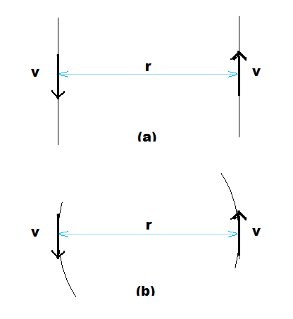
Fig (A1) shows two spinors passing. In case (a),the “rigidly-passing” vectors are not interacting, but they each see the other’s turning energy from Eqn. (1) as 2 v 0.866 ћ/r. In case (b), the vectors are interacting and the paths curve. The energy is actually less because the turning of each due to following the path(s) reduces the turning that each sees of the other. A “rigidly-passing” model, along with rules for how vector components in 3 dimensions see each other, is given in Appendix B. The normalized result is 2/3. The calculation of case (b) has been very difficult in practice and I have resorted to comparing nuclear models to experimental data to estimate Scale. The simplest, most symmetrical model in SOM context to use for this is the alpha particle.
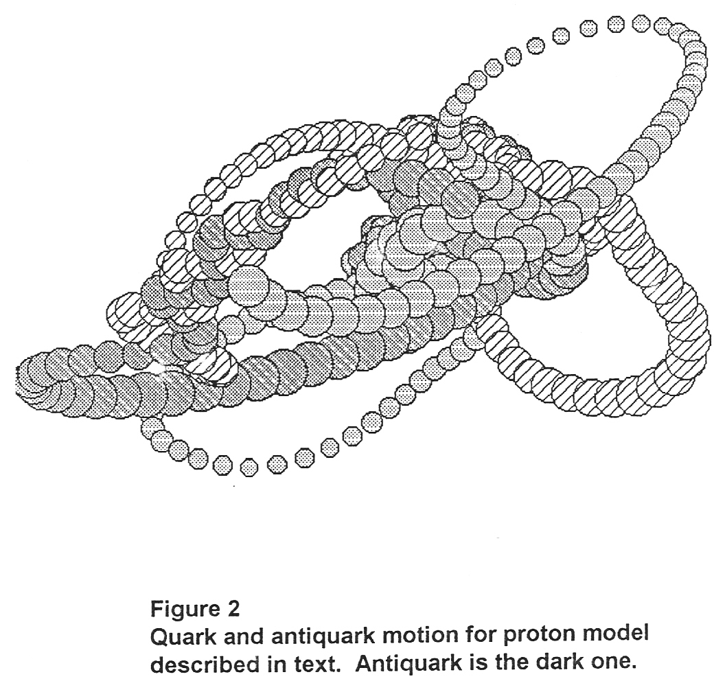
Fig (A2) shows a real-time model for one proton cycle. This was copied from “Nuclear Innards”, although copyrighted 2008, described SOM circa 1998.
So the scaling factor for the radius derived from the Compton wavelength equation is 196 MeV/fm, the “rigidly-passing” model gives 2/3 of that or 131 MeV/fm and the SOM alpha model gives half again or 65.5 MeV/fm.
Figure A1
Spin-Turning
EnergyTwo vectors passing:
(a) no interaction
(b) some interaction
separate image
Figure A2
Real-time
Proton Model 2 partics and an antipartic. Antipartic is darker
(no hidden line algorithm was used, so you
will have to imagine small circles are behind large ones)
larger image
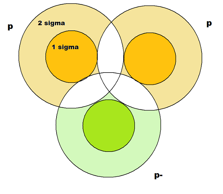
A nuclear bond in SOM is the attraction (negative potential) between p and p- due to Eqn. (1). A p is q q q-. A p- is q- q- q. All the combinations of Δv in three dimensions of q/q-, q/q and q-/q- add up to effectively one q/q- attraction between p and p- since the two q/q and two q-/q- combinations cancel 4 of the 5 q/q- combinations between a p and p-. I’ve used q to represent the partic spinor since it is somewhat quark-like and I need a letter different than p.
The 2 q/q- interactions and one q/q interaction within a p are the cause of the spread modeled by a Gaussian. Partic or antipartic paths that could be pictured as the outer layers of a ball of twine, with radius 0.5 to 0.6 fm, are spread into a ball of spaghetti with the same average radius. The p- is the same with opposite signs. Antibond is the name I use for the positive potential between p p or p- p-. The sum of bonds will be larger than the sum of antibonds for stable nuclei.
Figure 1
Proton and Antiproton
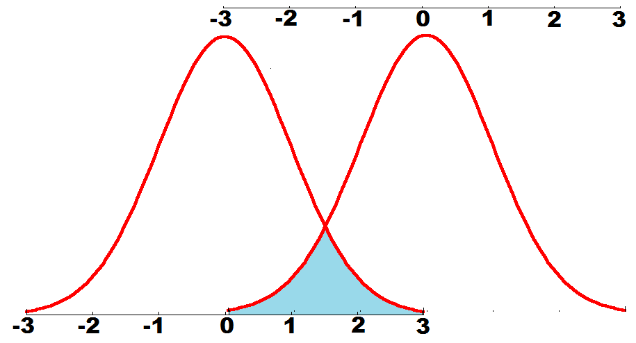
Overlap Statistics The scale is is σ-units
larger image
A slice through the bond overlap is shown in Fig. (1) for a p p- spacing of 3 σ-units. For a radius calibration of 0.866 “ideal”, 3 σ-units is about 2.1 fm. A top view is shown in Fig. (2) for the triton model to be discussed later.
Figure 2
Triton Model Overlaps
larger image
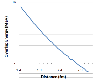
For the overlap region (shaded in blue in Fig. (1)) there is a possibility that a partic from the proton and an antipartic from the antiproton are on the opposite or wrong side of each other. (One q q- combination is used to represent the 9 combinations, 5 negative and 4 positive, that actually occur as described above.) In the case they are on the wrong side, the potential will reverse, lowering the potential that would otherwise be proportional to 1/r on the average. If Scale is the proportionality factor, then summing over all the possible 1/r factors from both the p and p- yields the results plotted in Fig. (3) for the overlap correction. This correction is the difference between 1/r and the average sum including the sign-reversed terms. A factor for Scale of 65.5 MeV/fm was used in the plot. Scale represents the sum over Δv in Eqn (1) and is assumed independent of r. There are independent models for Scale for estimating value ranges, but Scale, for the most part, will be determined by comparing alpha particle model parameters to alpha particle data.
Figure 3
Overlap Energy Scale=65.5 MeV/fm, σr=0.682 fm
larger image
p p bonds will use the same overlap corrections with opposite signs.
Summarizing: the potential of a p p- or p p bond is magnitude Scale/r with a correction for overlap as a function of r as given in Fig. (3). The current calibration for Scale is about 65.5 MeV/fm.